Older source codes
This page presents a list of older source codes developed at the Learning and Interaction Lab, Department of Advanced Robotics, Italian Institute of Technology (IIT), and at the Learning Algorithms and Systems Laboratory (LASA), Ecole Polytechnique Federale de Lausanne (EPFL).
Task-parameterized tensor GMM with missing frames

Demonstration a task-parameterized probabilistic model encoding movements in the form of virtual spring-damper systems acting in multiple frames of reference. Each candidate coordinate system observes a set of demonstrations from its own perspective. When one task parameter is not observable, the corresponding part in the data will be missing (third order sparse tensor data) and this information is taken into account in the learning and reproduction parts. The task is a via point passing task, starting from one point, passing through a second point and ending in a third point. A frame of references (task parameters) is attached to each via point, complemented by a fixed frame of reference at the origin.
Download
 Download task-parameterized tensor GMM with missing frames sourcecode
Usage
Unzip the file and run 'demo1' in Matlab.
Reference
- Alizadeh, T., Calinon, S. and Caldwell, D.G. (2014) Learning from demonstrations with partially observable task parameters. Proc. IEEE Intl Conf. on Robotics and Automation (ICRA).
Task-parameterized tensor GMM with LQR
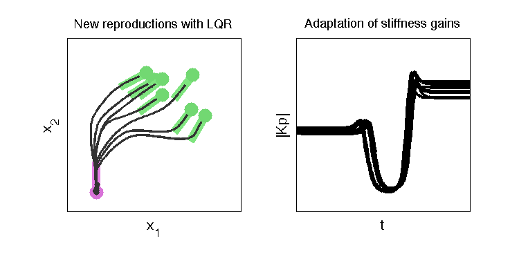
Demonstration a task-parameterized probabilistic model encoding movements in the form of virtual spring-damper systems acting in multiple frames of reference. Each candidate coordinate system observes a set of demonstrations from its own perspective, by extracting an attractor path whose variations depend on the relevance of the frame through the task. This information is exploited to generate a new attractor path corresponding to new situations (new positions and orientation of the frames), while the predicted covariances are exploited by a linear quadratic regulator (LQR) to estimate the stiffness and damping feedback terms of the spring-damper systems, resulting in a minimal intervention control strategy.
Download
Download task-parameterized tensor GMM with LQR sourcecode
Usage
Unzip the file and run 'demo01' in Matlab. Several reproduction algorithms can be selected by commenting/uncommenting lines 89-91 and 110-112 in demo01.m (finite/infinite horizon LQR or dynamical system with constant gains). 'demo_testLQR01' and 'demo_testLQR02' can also be run as examples of LQR.
Reference
- Calinon, S., Bruno, D. and Caldwell, D.G. (2014) A task-parameterized probabilistic model with minimal intervention control. Proc. of the IEEE Intl Conf. on Robotics and Automation (ICRA).
Task-parameterized GMM
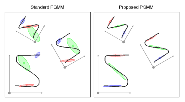
Training of a task-parameterized Gaussian mixture model (GMM) based on candidate frames of reference.
The proposed task-parameterized GMM approach relies on the linear transformation and product properties of
Gaussian distributions to derive an expectation-maximization (EM) algorithm to train the model.
The proposed approach is contrasted with an implementation of the approach proposed by Wilson and Bobick in
1999, with an implementation applied to GMM (that we will call PGMM) and following the model described in
"Parametric Hidden Markov Models for Gesture Recognition", IEEE Trans. on Pattern Analysis and Machine
Intelligence.
In contrast to the standard PGMM approach, the new approach that we propose allows the parameterization of
both the centers and covariance matrices of the Gaussians. It has been designed for targeting problems in
which the task parameters can be represented in the form of coordinate systems, which is for example the
case in robot manipulation problems.
Download
Download task-parameterized GMM Matlab sourcecode
Download task-parameterized GMM C++ (command line version) sourcecode
(see also DMP LEARNED BY GMR sourcecode)
Usage
For the Matlab version, unzip the file and run 'demo1' or 'demo2' in Matlab.
For the C++ version, unzip the file and follow the instructions in the ReadMe.txt file.
Reference
- Calinon, S., Li, Z., Alizadeh, T., Tsagarakis, N.G. and Caldwell, D.G. (2012) Statistical dynamical systems for skills acquisition in humanoids. Proc. of the IEEE Intl Conf. on Humanoid Robots (Humanoids).
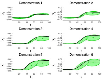
Demo 1 - Simple example of task-parameterized GMM learning and comparison with standard PGMM
This example uses 3 trajectories demonstrated in a frame of reference that varies from one demonstration to the other. A model of 3 Gaussian components is used to encode the data in the different frames, by providing the parameters of the coordinate systems as inputs (transformation matrix A and offset vector b).
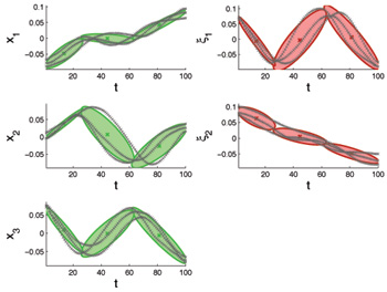
Demo 2 - Example of task-parameterized movement learning with DS-GMR (statistical dynamical systems based on Gaussian mixture regression)
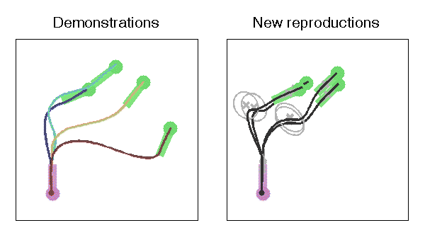
This demo shows how the approach can be combined with the DS-GMR model to learn movements modulated with respect to different frames of reference. The DS-GMR model is a statistical dynamical system approach to learn and reproduce movements with a superposition of virtual spring-damper systems retrieved by Gaussian mixture regression (GMR). For more details, see the 'DMP-learned-by-GMR-v1.0' example code downloadable from the website below.
DMP learned by GMR
Download
Download DMP learning with GMR Matlab sourcecode
Download DMP learning with GMR C++ (command line version) sourcecode
(see also TASK-PARAMETERIZED GMM sourcecode)
Usage
For the Matlab version, unzip the file and run 'demo1' in Matlab.
For the C++ version, unzip the file and follow the instructions in the ReadMe.txt file.
Reference
- Calinon, S., Li, Z., Alizadeh, T., Tsagarakis, N.G. and Caldwell, D.G. (2012) Statistical dynamical systems for skills acquisition in humanoids. Proc. of the IEEE Intl Conf. on Humanoid Robots (Humanoids).
Demo 1 - Simple example of DMP learning with GMR
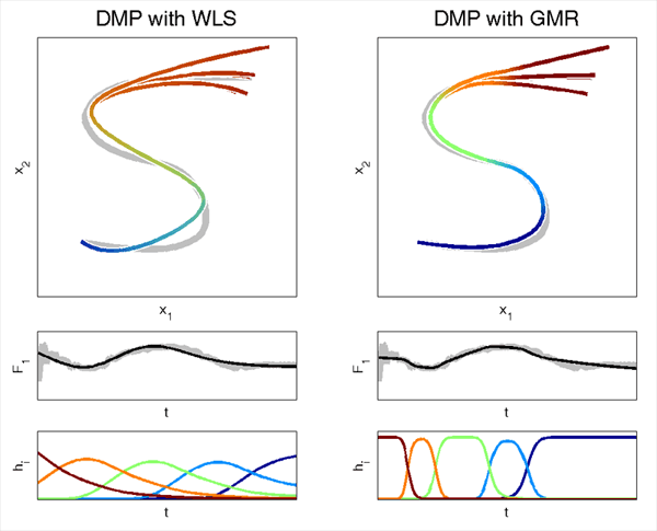
Simple example of estimating the parameters of a DMP (dynamic movement primitives) through GMR (Gaussian mixture regression).
A DMP is composed of a virtual spring-damper system modulated by a non-linear force.
The standard method to train a DMP is to predefine a set of activations functions and estimate a set of force
components through a weighted least-squares (WLS) approach.
The weighted sum of force components form a non-linear force perturbing the system,
by moving it away from the point-to-point linear motion while following a desired trajectory.
GMR is used here to learn the joint distribution between the decay term s (determined by a canonical dynamical
system) and the non-linear force variable to estimate.
Replacing WLS with GMR has the following advantages:
- It provides a probabilistic formulation of DMP (e.g., to allow the exploitation of correlation and variation information, and to make the DMP approach compatible with other statistical machine learning tools).
- It simultaneously learns the non-linear force together with the activation functions. Namely, the Gaussian kernels do not need to be equally spaced in time (or at predefined values of the decay term 's'), and the bandwidths (variance of the Gaussians) are automatically estimated from the data instead of being hand-tuned.
- It provides a more accurate approximation of the non-linear perturbing force with local linear models of degree 1 instead of degree 0 (by exploiting the conditional probability properties of Gaussian distributions).
Continuous HSMM
Download
Download Continuous HSMM sourcecode
Usage
Unzip the file and run 'demo1' in Matlab.
Reference
- Calinon, S., Pistillo, A. and Caldwell, D.G. (2011) Encoding the time and space constraints of a task in explicit-duration hidden Markov model. Proc. of the IEEE/RSJ Intl Conf. on Intelligent Robots and Systems (IROS).
Demo 1 - Simple example of continuous HSMM
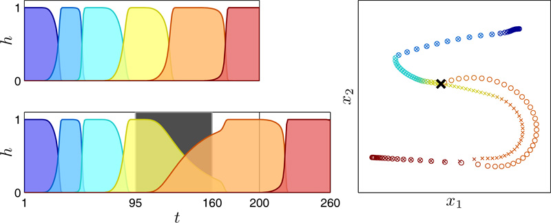
Simple example of the use of Hidden Semi-Markov Model (HSMM), a form of explicit-duration Hidden Markov model, to learn and reproduce trajectories.
The movement is represented as a combination of linear systems with a velocity dx computed iteratively as dx = sum_i h_i (A_i x + b_i), where h_i is a weight defined by HSMM.
A_i and b_i form a matrix and vector associated with state i of the HSMM.
Rescaled GMM
Download
Download Rescaled GMM sourcecode
Usage
Unzip the file and run 'demo1' in Matlab.
Reference
- Pistillo, A., Calinon, S. and Caldwell, D.G. (2011) Bilateral Physical Interaction with a Robot Manipulator through a Weighted Combination of Flow Fields. Proc. of the IEEE/RSJ Intl Conf. on Intelligent Robots and Systems (IROS).
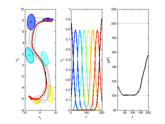
Demo 1 - Simple example of Rescaled GMM
Simple example of using a Gaussian Mixture Models (GMMs) to learn and reproduce movements represented as a combination of linear
systems with a velocity command dx computed iteratively as dx = sum_i h_i (A_i x + b_i), where A_i and b_i form a matrix and vector associated with state i of the GMM.
The novelty here is that h_i is a weight originally defined by GMM and rescaled during reproduction to authorize motion commands only in the regions of the task demonstrations, while the movemement fades away outside those (according to the task constraints, that is, local variability).
With the new weighting mechanism, each linear subsystem becomes independent from the others.
Correlated DMP
Download
Usage
Unzip the file and run 'demo1' in Matlab.
Reference
- Calinon, S., Sardellitti, I. and Caldwell, D.G. (2010) Learning-based control strategy for safe human-robot interaction exploiting task and robot redundancies. Proc. of the IEEE/RSJ Intl Conf. on Intelligent Robots and Systems (IROS).
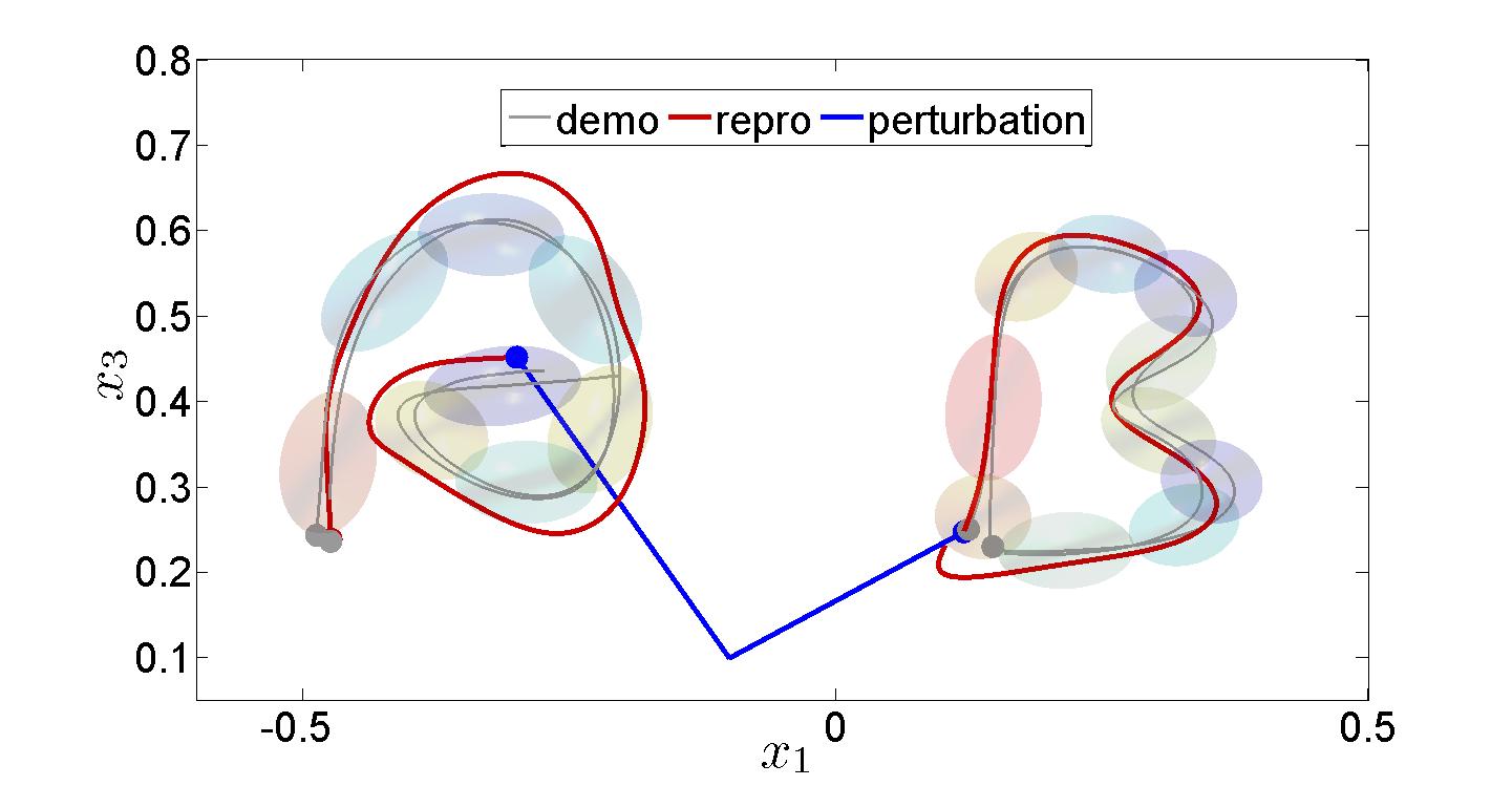
Demo 1 - Mixture of correlated mass-spring-damper systems
Learning and reproduction of a movement through a mixture of dynamical
systems (similar to Dynamic Movement Primitives), where variability and correlation information along the movement and among the different examples is encapsulated as a full stiffness matrix in a set of mass-spring-damper systems.
For each primitive (or state), learning of the virtual attractor points
and associated stiffness matrices is done through least-squares regression.
GMR Dynamics
Download
Â
Download GMR Dynamics sourcecode
Usage
Unzip the file and run 'demo1' in Matlab.
Reference
- Calinon, S., D'halluin, F., Sauser, E.L., Caldwell, D.G. and Billard, A.G. (2009) A probabilistic approach based on dynamical systems to learn and reproduce gestures by imitation. IEEE Robotics and Automation Magazine.
Demo 1 - Demonstration of a trajectory learning system robust to perturbation based on Gaussian Mixture Regression (GMR)
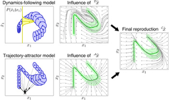
This program first encodes a trajectory represented through time 't', position 'x' and velocity 'dx'
in a joint distribution P(t,x,dx) through Gaussian Mixture
Model (GMM) by using Expectation-Maximization (EM) algorithm. Gaussian Mixture Regression (GMR)
is then used to estimate P(x,dx|t), which retrieves another GMM refining the joint distribution
model of position and velocity.
The learned skill can then be reproduced by combining an estimation of P(dx|x)
with an attractor to the demonstrated trajectories.
Joint/task constraints
Download
Â
Download Joint/task constraints sourcecode
Usage
Unzip the file and run 'demo1' in Matlab.
Reference
- Calinon, S. and Billard, A. (2008) A Probabilistic Programming by Demonstration Framework Handling Constraints in Joint Space and Task Space. IEEE/RSJ International Conference on Intelligent Robots and Systems (IROS), pp. 367-372.
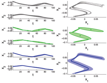
Demo 1 - Demonstration of the use of Gaussian Mixture Regression (GMR) and inverse kinematics to reproduce a task by considering constraints both in joint space and in task space

This program shows the simulation of a robotic arm composed of 2 links and moving in 2D space.
Several demonstrations of a skill are provided, by
starting from different initial positions. The skill consists of moving
each joint sequentially and then writing the alphabet letter 'N' at a
specific position in the 2D space.
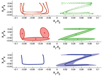
Constraints in joint space and in task space are represented
through Gaussian Mixture Models (GMMs) and Gaussian Mixture Regression
(GMR). By using an inverse kinematics process based on a pseudo-inverse
Jacobian, the constraints in task space are then projected in joint
space. By considering the projected constraints with the ones originally
encoded in joint space, an optimal controller is found for the
reproduction of the task. We see through this example that the system is
able to generalize the learned skill to new robotic arms (different links
lengths) and to new initial positions of the robot.
Cone-plane intersection
Download
Â
Download Cone-plane intersection sourcecode
Usage
Unzip the file and run 'demo1' in Matlab.
References
- Calinon, S. and Billard, A. (2006) Teaching a Humanoid Robot to Recognize and Reproduce Social Cues. IEEE International Symposium on Robot and Human Interactive Communication (RO-MAN), pp. 346-351.
Demo 1 - Demonstration of a cone-plane intersection interpreted in terms of Gaussian Probability Density Function (PDF)

This program computes the intersection between a cone and a plane, represented as a Gaussian Probability Density Function (PDF). The algorithm can be used to extract probabilistically information concerning gazing or pointing direction. Indeed, by representing a visual field as a cone and representing a table as a plane, the Gaussian distribution can be used to compute the probability that one object on the table is observed/pointed by the user.
GMM incremental learning
Download
Â
Download GMM incremental sourcecode
Usage
Unzip the file and run 'demo1' or 'demo2' in Matlab.
References
- Calinon, S. and Billard, A. (2007) Incremental Learning of Gestures by Imitation in a Humanoid Robot. Proceedings of the ACM/IEEE International Conference on Human-Robot Interaction (HRI), pp. 255-262.
Demo 1 - Demonstration of an incremental learning process of Gaussian Mixture Model (GMM) using a direct update method
The demonstration loads a dataset consisting of several trajectories which are presented one-by-one to update the GMM parameters by using an incremental version of the Expectation-Maximization (EM) algorithm (direct update method). The learning mechanism only uses the latest observed trajectory to update the models (no historical data is used).
Demo 2 - Demonstration of an incremental learning process of Gaussian Mixture Model (GMM) using a generative method
The demonstration loads a dataset consisting of several trajectories which are presented one-by-one to update the GMM parameters by generating stochastically a new dataset from the current model, adding the new trajectory to this dataset and updating the GMM parameters using the resulting dataset, through a standard Expectation-Maximization (EM) algorithm (generative method). The learning mechanism only uses the latest observed trajectory to update the models (no historical data is used).
GMR multiple constraints
Download
Â
Download GMR multiConstraints sourcecode
Usage
Unzip the file and run 'demo1' in Matlab.
References
- Calinon, S. and Billard, A. (2007) What is the Teacher's Role in Robot Programming by Demonstration? - Toward Benchmarks for Improved Learning. Interaction Studies. Special Issue on Psychological Benchmarks in Human-Robot Interaction. 8:3, 441-464.
Demo 1 - Demonstration of the reproduction of a generalized trajectory through Gaussian Mixture Regression (GMR), when considering two independent constraints represented separately in two Gaussian Mixture Models (GMMs)

Through regression, a smooth generalized trajectory satisfying
the constraints encapsulated in both GMMs is extracted, with associated
constraints represented as covariance matrices.
The program loads two datasets, which are encoded separetely in two
GMMs. GMR is then performed separately on the two datasets, and the
resulting Gaussian distributions at each time step are multiplied to
find an optimal controller satisfying both constraints, producing a
smooth generalized trajectory across the two datasets.
GMM latent space
Download
Â
Download GMM latent space sourcecode
Usage
Unzip the file and run 'demo1' in Matlab.
References
- Calinon, S. and Billard, A. (2005) Recognition and Reproduction of Gestures using a Probabilistic Framework combining PCA, ICA and HMM. In Proceedings of the International Conference on Machine Learning (ICML), pp. 105-112.
Demo 1 - Demonstration of a probabilistic encoding through Gaussian Mixture Model (GMM) in a latent space of motion extracted by Principal Component Analysis (PCA)
This programs loads a dataset, finds a latent space of lower dimensionality encapsulating the important characteristics of the motion using Principal Component Analysis (PCA), trains a Gaussian Mixture Model (GMM) using the data projected in this latent space, and projects back the Gaussian distributions in the original data space. Training a GMM with EM algorithm usually fails to find a good local optimum when data are high-dimensional. By projecting the original dataset in a latent space as a pre-processing step, GMM training can be performed in a robust way, and the Gaussian parameters can be projected back to the original data space.
GMM-GMR
Download
Usage
Unzip the file and run 'demo1', 'demo2' or 'demo3' in Matlab.
References
- Calinon, S., Guenter, F. and Billard, A. (2007) On Learning, Representing and Generalizing a Task in a Humanoid Robot. IEEE Transactions on Systems, Man and Cybernetics, Part B. 37:2, 286-298.
Demo 1 - Demonstration of the generalization process using Gaussian Mixture Regression (GMR)
The program loads a 3D dataset, trains a Gaussian Mixture Model (GMM), and retrieves a generalized version of the dataset with associated constraints through Gaussian Mixture Regression (GMR). Each datapoint has 3 dimensions, consisting of 1 temporal value and 2 spatial values (e.g., drawing on a 2D Cartesian plane). A sequence of temporal values is used as query points to retrieve a sequence of expected spatial distribution through Gaussian Mixture Regression (GMR).
Demo 2 - Demonstration of Gaussian Mixture Regression (GMR) using spatial components as query points of arbitrary dimensions
The programs loads a 4D dataset, trains a Gaussian Mixture Model (GMM), and uses query points of 2 dimensions to retrieve a generalized version of the data for the remaining 2 dimensions, with associated constraints, through Gaussian Mixture Regression (GMR). Each datapoint has 4 dimensions, consisting of 2x2 spatial values (e.g., drawing on a 2D Cartesian plane simultaneously with right and left hand). A new sequence of 2D spatial values (data for left hand) is loaded and used as query points to retrieve a sequence of expected spatial distribution for the remaining dimensions (data for right hand), through Gaussian Mixture Regression (GMR).
Demo 3 - Demonstration of the smooth transitions properties of data retrieved by Gaussian Mixture Regression (GMR)

This program loads two 3D datasets, trains two separates Gaussian Mixture Model (GMM), and retrieves a generalized version of the two datasets concatenated in time, with associated constraints, through Gaussian Mixture Regression (GMR). Each datapoint has 3 dimensions, consisting of 1 temporal value and 2 spatial values (e.g., drawing on a 2D Cartesian plane). A sequence of temporal values is used as query points to retrieve a sequence of expected spatial distribution through Gaussian Mixture Regression (GMR). The position of the last datapoint in the first dataset is not consistent with the first datapoint of the second dataset. However, by encoding separately the two datasets in GMM and concatenating the components in a single model, a smooth signal with smooth transition between the two data is retrieved through regression.